Juniper publishers Implementation of A* Algorithm to Autonomous Robots-A Simulation Study
Juniper Publishers - Open Access Journal of Engineering Technology
Authored by : Selvakumar AA
Abstract
This article presents some of the current
contributions to the robotic path planning field. Reliable collision
free path is the fundamental thing for proper working of autonomous
vehicle/robots. In order to find an optimal path for robot, environment
or workspace need to be understood correctly and suitable algorithm need
to used. Many researchers developed different algorithm techniques as
per the required operations. This paper presents an overview of strength
and weakness of A* algorithm for static environment using distance
formula. A* algorithm works on the lower details of the map hence, it is
considered as a higher-level path planning technique. A* algorithm is
based on the availability of adjacent nodes and distance of goal
location from the current state of the robot.
Keywords: A* algorithm; Path planning; Hierarchical algorithms; Heuristics Introduction
Autonomous robots attained genuine attention because
of variety of applications in the household, industrial as well as
military purpose. For the accurate performance of such mobile robots,
navigation or motion planning is the key aspect. It includes perception
of environment based on sensory data, configuring with the surrounding
and decision making which is an important phase to find an optimal path
from the start location to the goal location without any collision with
the surrounding. Different algorithm techniques have been used the path
planning of autonomous robots. For example, genetic algorithm,
grid-based algorithms, geometry-based algorithms, sampling-based
algorithms. Most commonly used technique for static environment is
grid-based algorithm. It includes configuration space which is divided
into no. of small grids and hence detecting the obstacles robot finds
the path from start location to goal location in the configuration
space. But, in order to find the optimum solution, i.e. collision free
path with the shortest distance so as to minimize the travel time,
distance formula is implemented with the A* algorithm [1].
A* algorithm is grid-based path planning technique.
Basically, A* algorithm was initially designed for the graph transversal
problems. Later, it was commonly used for path finding applications
such as computer games. A* algorithm is practically easier and faster
for implementation [2].
A* algorithm is suitable for the static environments only. Also, it is
not good for obstacle shape changes. To reach the goal position, A*
algorithm creates sub optimal paths with the help of neighboring grids.
It is represented as f (n) = g (n) + h'(n) where, g (n) is the distance from the start position to the current position whereas h'(n)
is the estimated distance from current state to the goal position. In
order to find this estimation heuristic function is used. f(n)
is nothing but the estimated shortest path from the start location to
the goal destination. In this technique, distance formula is used as a
heuristic function [3].
In practical situation, static environment may be
large for this algorithm to solve. Such cases are solved by defining a
hierarchical solution. A* algorithm works on probability-based maps,
i.e., it always tries to find path with the smallest length having
lowest probability of the collision with the surrounding. Here path
length factor is dominant one. [3] Also, as the obstacle size increases probability of collision with the surrounding reduces drastically. [4]
Stated in their article, A* algorithm is not suitable for the static
environment with the smaller size obstacles as this algorithm tends to
find shortest path only over the obstacle avoidance.
Problem Statement
In the static environment, position or orientation of
the obstacles are not changing. Hence configuration space is considered
as a rectangular terrain, which can be divided into number of small
grid. Initial and final location of robot or obstacles can be
represented in these grids. Here, the problem is considered as a
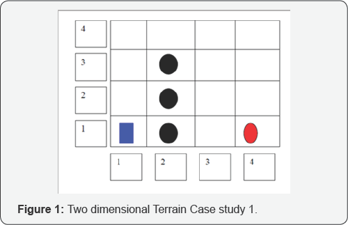
two-dimensional transverse terrain shown in the following Figure 1.
As shown in the Figure 1,
configuration space is divided into number of grids. Autonomous robot
is represented by blue dot. It has to transverse the terrain and reach
the goal location which is represented by red oval. Black dots represent
the obstacles.
Algorithm Guidance
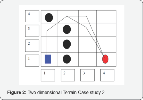
Consider the case of a 4x4 configuration space. The
starting node is (1,1). The successive node is only one in this case
which is (1,2). There is no confusion, until the Robot reaches node
(2,4). Now, there are two nodes (3,4) and (3,3). The successor node can
be determined by evaluating the cost to the target from both the nodes (Figure 2).
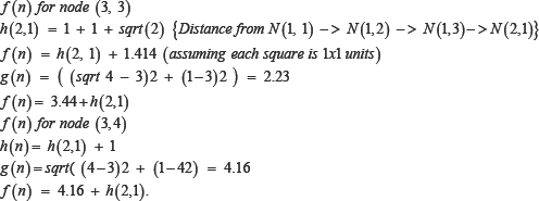
Now, f (n) for (3,3) is smallest of the two, hence the successor node is f (n)
. The robot can now transverse to the node (3, 3) and continue
expanding the successor nodes as above, until the goal location is
reached.
Consider a configuration with dead end condition (Figure 3).
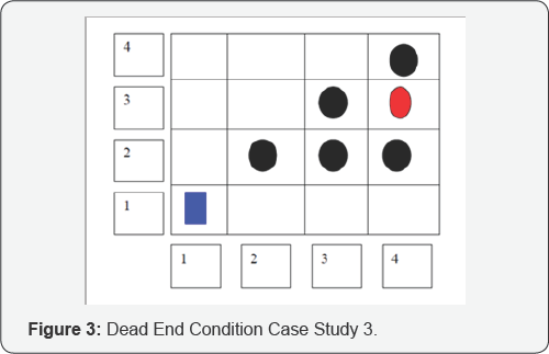
Here, from Node (2,1) will be chosen as the successor
node instead of Node (1,2). The robot will continue to traverse the
route until it ends up at the block at Node (4,1). Here, need to add an
algorithm by which the robot find outs alternate paths once it ends up
at a dead node (dead end). Avoids traversing paths that follows to a
dead node.
This is achieved by keeping up two records OPEN and
CLOSED. OPEN list contains successive paths that are yet to be computed
and CLOSED list is having all paths that have been explored. The list
OPEN also stores the parent node of current location. This is used at
the end to trace the path from the Goal to the Start position, thus
calculating the optimum path. The start node has 2 successors (2,1) and
(1,2). From the initial calculation (2,1) is chosen and the robot
travels along that node, however ones it reaches the dead end, it
discards the node (2,1) and takes the second successor (1,2) and
explores that route Figure 4.
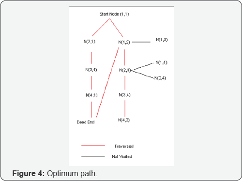
Once the goal location is reached the parent nodes
are highlighted and tracked back to the start location to get the
complete path. In the above example N(4,3),N(3,4), N(2,3), N(1,2),
N(1,1) gives the optimum path. From the above conditions the following
algorithm is obtained [3].
Algorithm Flow
Consider the first node and put it to the OPEN list. As it is the start point, is zero.
Now, next adjacent node's cost function is calculated. Smallest one is shifted to CLOSED list.
Suppose, robot reach to goal location, stop the
algorithm. With the help of all cost functions, determine the path
value. Otherwise, continue with the next nodes.
In the same manner, compute the cost function for all adjacent nodes with respect to robot's current position.
Now, with respect to parent node, sort the successor
nodes to OPEN or CLOSED lists. Repeat the cycle till cost function of
current location is zero (Distance between current location and goal
becomes zero).
Simulation
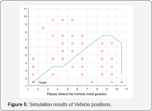
Simulation is carried out using MATLAB. Based on
MATLAB coding, two-dimensional array of a configuration space is
created. Autonomous robot's initial location and goal location we can
assigned. Obstacles are assigned manually. From these above inputs we
got the output as Figure 5.
Result
Hence, the optimum path is found out from start
location to the goal location in a static environment using
classification of open nodes and closed nodes based upon distance
formula. This technique is successfully implemented to the different
static environments as far as obstacles are in its definite shape and
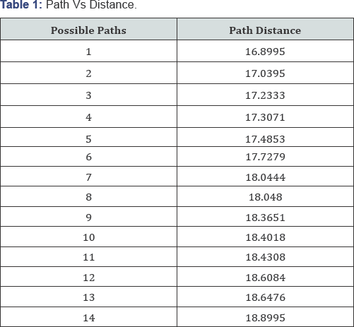
size. If we consider each grid of dimension 1x1 unit, following are the
results from the simulation of the total distance of some possible paths
[5-11]. From the results shows in Table 1, the available shortest path is highlighted in the Figure 5.
Summary
Hence, A* algorithm is successfully implemented to
the static environment using MATLAB simulation. This technique of path
planning finds the optimal path with respect to the distance, but
practically there are chances of collision with the surroundings as
distance is the dominating factor in this algorithm over obstacle
avoidance. In order to serve this purpose, more accurate understanding
of the environment is essential. Also, to get more optimum results with
respect to distance, integration of this technique with neural network
can be used. Future scope in this area refers to integration of this
algorithm with genetic algorithm, i.e., simulation results of this
algorithm can be treated as an initial population for genetic method for
determining more optimized path.
For more articles in Open Access Journal of
Engineering Technology please click on:
https://juniperpublishers.com/etoaj/index.php


Comments
Post a Comment